Arduino CW decoder
Mar 2021
Since completing the oscilloscope project I have been working on a CW (Morse code) decoder. After trying 5 different designs and techniques I have finally homed in on a solution that works well. This video shows an early prototype decoding a Titanic message video on YouTube.
Using the Arduino as a starting point meant I could use the knowledge of hardware and software that I had developed whilst working on the oscilloscope. Some of the issues I encountered could have been mitigated by using more processing power but I was enjoying the challenge of working around the limitations of memory and speed so I persevered with the Arduino.
With this in mind, my initial thought was to reduce the processing load by using hardware to separate the signal from the carrier. After some simulation and testing of low pass filters, I decided that this approach was not feasible and would result in too much distortion of the wanted signal.

The main limitations of the Arduino Uno R3 specification were:
The analog to digital converter (ADC) is relatively slow.
Driving displays takes a lot of time and memory (especially if using the published libraries)
2kB of RAM is very restrictive for processing dynamic data.
Audio Sampling
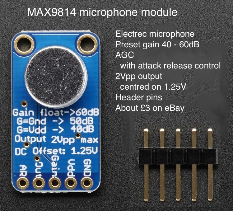
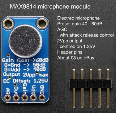
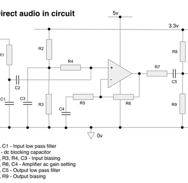
The next step was to feed a sample CW signal into the Arduino ADC for software processing. To do this I used a MAX9814 microphone module and a simple op amp circuit to amplify the signal.
For sample signals I turned to YouTube where there is a wide range of training videos and actual CW contact recordings.
My Arduino oscilloscope allowed me to visualise the signal but I also used a new feature of the Arduino IDE - a serial link plot function. This runs on the host computer and takes the serial print output of the Arduino and plots it on a chart rather than just printing it out. However, at this point the limitations of the Arduino became apparent.
The ADC takes around 15 μs and serial print takes over 100 μs to print an integer. This limits a real time display to a maximum frequency of around 2kHz (using a sampling rate of twice the signal frequency).
Alternatively, the samples can be stored in an array and printed out in batches. This allows frequencies up to around 12kHz to be displayed but the 2kB ram can only store about 500 samples. Still, working between these limits with suitable triggering gave a useful view of the signal to be processed. This was invaluable for fault finding and diagnostics.
Signal Processing
A simple analysis of the analog signal samples was sufficient to identify when the carrier was present but this approach was easily defeated by background noise and changes in volume. Clearly a better solution would be to digitally extract the amplitude of the carrier frequency which pointed me in the direction of the Discrete Fourier Transform (DFT).
I spent a lot of time finding out how DFT worked and simulating it on Excel to find the best combination of sampling frequency and number of samples. The number of samples equals the number of "bins" for the frequency amplitude measurements. Each bin is a centre frequency for which the amplitude can be captured. Only half the bins can be used (ie sampling frequency must be at least twice the target frequency. However the number of samples also determines the accuracy of the measurements.
The Fourier calculations can be simplified by solving for a single target frequency using the Goertzel algorithm and ignoring the imaginary part of the signal. This worked equally well in the simulation and was much easier to process on the Arduino.
To use DFT on a waveform it needs to have positive and negative values about a zero reference point. The Arduino ADC works with a positive voltage and gives a value from 0 - 1023. This was resolved by taking the average value of the waveform over time and using that value as the zero reference point. This was then subtracted from each sample before the DFT processing.
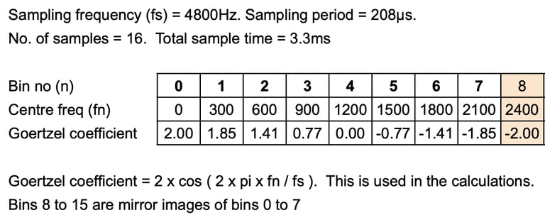
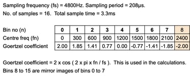
I started with around 11,500 samples per second and 50 samples which gives a measurement time of 4.5ms snd a bin size of 230Hz. Although this worked well in the Excel simulation, I couldn't replicate the results on the Arduino and I eventually realised that the floating point calculations were taking too long and disrupting the sampling speed. To solve this I took the sampling rate down to 4,800 samples per second and used 16 samples to give a measurement time of 3.3ms and a bin size of 300Hz.
This configuration gave a workable CW signal that I could now start decoding
Raferences
By far the best description of DFT that I found was an article in Practical Cryptograph:
The Goertzel algorithm is explained well in Wikipedia:
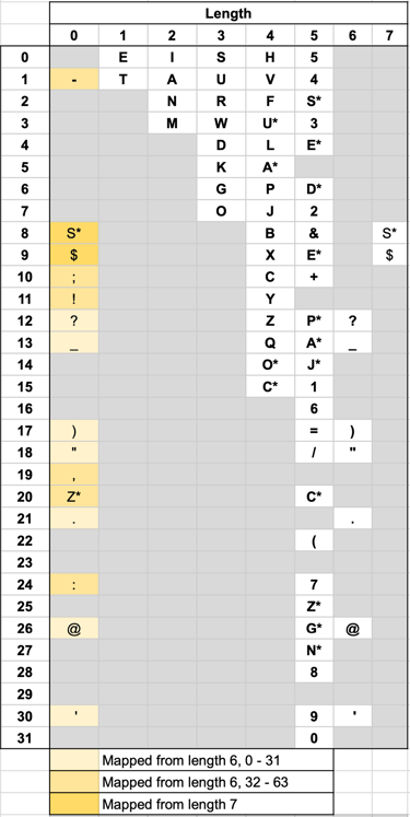
Morse code is unusual in that there is no fixed length for a character - the number of symbols (dots/dashes) ranges from 1 to 7. If we consider a dot to be represented by a binary 0 and a dash by 1 then all possible combinations can be represented by using 7 bits of a byte giving 127 values. However, these values would not be unique - for instance E, I, S, H and 5 would all have the value 0. Therefore the number of symbols also needs to be taken into account.
I created a 2 dimensional array to map characters to the dot/dash combinations. I started with a 128 x 7 array which caters for all the characters encoded into a length of up to 7 symbols. This would reserve 896 bytes of memory, much of which is not used - for instance, the 1 symbol characters only need 2 values (E and T), the 2 symbol characters 4, etc.
As a compromise between memory usage and processing speed I mapped the 6 and 7 symbol characters into column zero of the array. Fortunately this could be done without any clash of values as shown in the table. The result is a 32 x 6 array which saves over 700 bytes but is simple to process.
Morse Code
The next step was to develop the software to translate the processed signal into characters and word breaks.
Morse code is unusual in that there is no fixed length for a character - the number of symbols (dots/dashes) ranges from 1 to 7. If we consider a dot to be represented by a binary 0 and a dash by 1 then all possible combinations can be represented by using 7 bits of a byte giving 127 values. However, these values would not be unique - for instance E, I, S, H and 5 would all have the value 0. Therefore the number of symbols also needs to be taken into account.

Timing
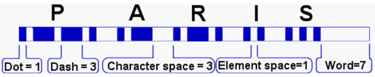
To determine whether the signal is a dot or a dash, the decoding algorithm needs to know how long the signal is high for and to determine when a character ends and when a word ends it also needs to know how long the signal is low for.
The unit of time used for these measurements is the length of a dot which I will call 1 bit time. All other Morse code timings are multiples of this bit time as listed in the example below.

As there is no timing signal in Morse code, the bit time needs to be determined before the signal can be decoded. The first version of my decoder monitored the signal for a few seconds before starting to decode. This allowed the shortest high/low state to be found and assumed this to be 1 bit time. However, the disadvantage of this approach is that the timing will change - both during a transmission and when switching to another signal. An additional timing algorithm was needed to dynamically adapt when the timing varied.
The result was a sampling algorithm that detected high-low and low-high changes of state and measured the time between them. These were used to maintain a moving average bit time against which the high/low time was compared:
High time < 2 x bit time = dot
High time > 2 x bit time = dash
Low time < 2 x bit time = element space
Low time > 5 x bit time = word space
Low time between 2 x bit time and 5 x bit time = character space
The accuracy of the bit timing was limited by the sampling time of 3.3ms. At 20 words per minute, the nominal bit time is 60ms which gives 5% uncertainty for each edge detection which is not a problem but it would become more significant at higher transmission rates.
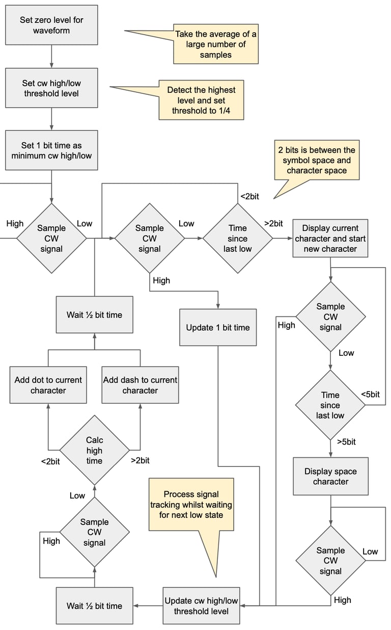
The sampling could not be run continuously as I needed processing time for other activities. I therefore waited half a bit time from the last transition before starting to sample for the next transition. The resulting high level software flow chart is shown below.

Development
With the decoder now working reasonably well, I started looking for solutions to some of the shortcomings that I had identified. These ranged from simple changes to a complete rethink of the methodology!
The limitations fell into 3 main categories
Waveform processing
Variations in CW speed and quality
User interface
Waveform Processing
The main issue with the decoder was that whilst it worked well on the sample 20wpm practice video that I had used in development, it struggled with other examples. I guessed that the Discrete Fourier Transform (DFT) algorithm was mainly to blame as this had a fixed centre frequency of 600Hz. To compensate it had a relatively wide bandwidth (around 300Hz) but this was quite wide for filtering out noise and too narrow for some of the carrier frequencies in use.
I looked at different sampling speeds and numbers of samples combined with a calibration routine to identify the best centre frequency. This helped but wouldn't adapt to a change of carrier frequency without a recalibration. I looked at sampling adjacent centre frequencies whilst waiting between samples but this was not very successful and took too long. I even looked at other techniques including monitoring the amplitude of the carrier directly or timing the carrier cycles to pick up the presence or absence of signal. Both of these worked to an extent but I eventually concluded that the benefits of the DFT approach far outweighed the limitations.
As a diversion whilst pondering how to improve the DFT solution, I built a simple interface to bypass the microphone and connect the computer headphone output directly to the decoder. I did this primarily to remove the background household noises and to avoid my wife's complaints of "annoying" tones from the computer. However, I was pleasantly surprised to find that it also solved most of the variation in signal level issues. I believe that the small room where I was doing the testing with the microphone was echoing and/or resonating certain frequencies and resulting in changes in level as I moved about and altered the resonances.
So, I decided the best way forward was to run the Analogue to Digital Converter (ADC) measurements and DFT calculations continuously with a variable sampling rate that adapted to the carrier frequency.
I also decreased the DFT sampling rate and increased the number of samples to narrow the bandwidth of the target frequency. This would normally result in the sampling taking too long so I ran 4 DFT calculations in parallel with the outputs spaced evenly in time. With some experimentation and tuning this technique provided a much better solution but it also introduced a lot of new timing constraints that meant that I had to completely restructure the coding - more on this later.
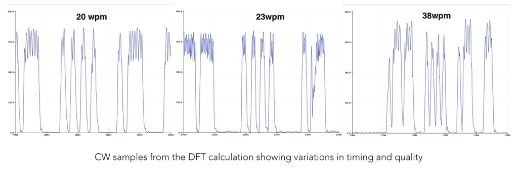
CW speed and quality variations
With a direct audio input and the revised DFT processing algorithm, the CW signal output was now much cleaner. The large variations in high state amplitude were no longer apparent, the noise level was reduced and the shape of the pulses much better defined.
However, it was still necessary to adapt to the CW speed to ensure that the dots and dashes could be discriminated and the inter symbol spaces correctly identified. This was made more difficult as the low state bit time could be as little as half the high state bit time or as large as twice the high state bit time. Similarly, some of the inter character spaces could be greater than 3 low state bit times and the inter word spaces less than 7 low state bit times.
My initial calibration approach was not that useful for this issue and a more adaptive system was necessary. This will be described in more detail later.
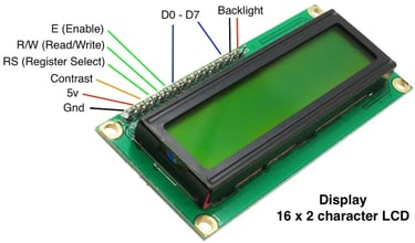
User Interface
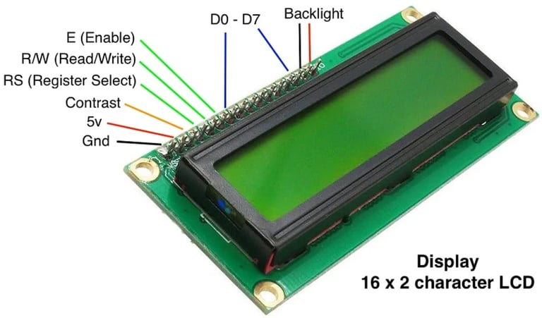
A simple 16 character x 2 line LCD display was chosen to display user messages and the decoded CW characters. As with the OLED display used for the oscilloscope project, the available libraries were slow and took up a lot o memory with features that are not needed for a simple implementation. However, the advantage of the LCD display over the OLED is that the character mapping is held in the LCD memory so it is not necessary to define fonts and send every pixel to the device - just the required character code. It also has a scroll mode such that each new character moves the display across automatically.
With reference to the datasheet and some trial and error, I wrote a short setup routine to initialise the LCD display and set up the relevant parameters. This allowed me to display a character in around 90 μs compared with around 1.6 ms to display a character on the OLED display.
I used the 4 bit data transfer mode to save data pins on the Arduino although this made the data transfer a little more involved. I intended to use both lines of the display but this would have meant I couldn't use the automatic scrolling in the way I wanted so I reverted to a single line display.
Programming
As hinted above, the latest version of the software moves away from the simple process flow described above and is now orientated around the need to sample the waveform continuously and sufficiently fast enough to measure the frequency of the carrier. All the other processing had to be slotted in between the sampling without affecting the timing.
The sampling rate needed to be as fast as practical in order to allow the carrier frequency to be measured with sufficient accuracy. Assuming a starting carrier frequency of 600Hz, I chose to run the ADC at 19,200 samples per second which gives a nominal frequency measurement accuracy of about 5%. However, this gives a 52 μs period in which to do the sampling and any other processing before taking the next sample. This is somewhat challenging to say the least!
The other advantage of continuous sampling is that the DFT process can now be run continually. This allows multiple DFT processes to be run in parallel to produce an output at regular intervals whilst still capturing sufficient samples to narrow the bandwidth and improve the signal quality.
I used every 8th ADC measurement as an input to the Goertzel DFT algorithm which gave 2,400 samples per second. Using 32 samples for each Goertzel output, this gave a much more focussed 75Hz bandwidth at a rate of 75 output measurements per second. This would allow just 4 DFT values within a "bit" period at 20wpm so I ran 4 DFT processes in parallel giving 300 output measurements per second which should be adequate up to around 60wpm.
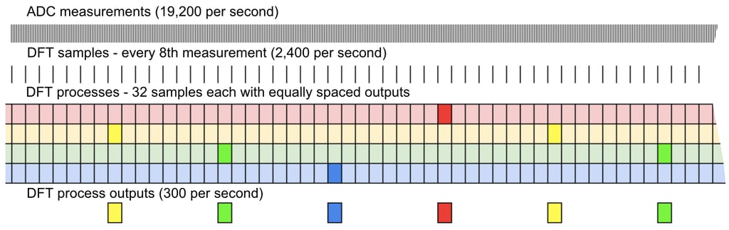
There was another good reason for choosing these sampling values for the Goertzel algorithm: for a 600Hz carrier, the coefficient used in the calculation becomes zero. This means that the calculation is much simpler and does not require floating point arithmetic which reduces the processing time by an order of magnitude. This was essential in order to fit the processing into the 52 μs period dictated by the ADC measurement cycle.
This still leaves the problem of adjusting the DFT sampling for carrier frequencies other than 600Hz which I discuss below.
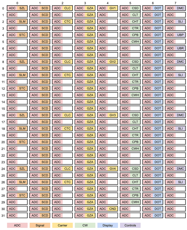
In the actual code there are just 8 scheduling segments, represented as a row in the matrix. Each segment contains the Analog to Digital conversion (ADC) module and 1 other. These are all run 32 times (as per the columns) before the sequence returns to the start. The current row is defined by a counter which is used to determine which modules to execute in that row.
The modules fall into 6 main categories which I have colour coded in the diagram. The individual modules in each category split the overall objective into sections of code that can run in a timeslot without exceeding the sampling time interval. I used counters and flags to provide continuity between modules and ensure they were run in the correct order. I will give an overview of each category with a few examples of the individual modules.
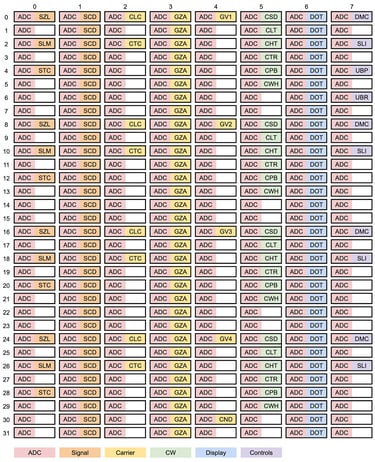
Program Schedule
This section describes the structure of the programming and the adaptations necessary to make it work within the limited processing power of the Arduino. There are other, faster, processors available but, for me, the enjoyment of this project is in finding solutions within the limits.
To create the program structure, I defined 256 "timeslots" that repeat sequentially and continuously once the set up tasks have been completed. In order to visualise this I imagined it as a matrix of 8 columns and 32 rows as shown below.
ADC
The ADC samples the signal in every timeslot and provides the input value into other modules. The raw signal is a voltage in the range 0 - 3.3v and this gives an integer in the range 0 - 1023. The module subtracts the zero level value (initially determined in the setup) to give the positive and negative waveform values required by the Goertzel algorithm.
This module also records the maximum input signal every 16 samples to provide a peak value that can be used to keep track of the volume and a running total to allow an average value to be calculated to track any changes in the zero level.
Signal
The most important module in this category is the carrier detection (SCD) which times the interval between zero level crossing points and looks for consistent values that indicate a carrier tone. This frequency is then calculated and passed to the carrier processing modules.
The carrier detection module is supported by signal level and zero level monitoring modules that set the threshold for measuring a signal zero level crossing. The signal level measurement module introduces a delay to the incoming signal to allow time for any threshold changes to take effect before the CW detection processes see the output carrier
level. It also attempts to distinguish a valid signal from noise and apply a digital "squelch" to suppress spurious output when the noise level is high.
Carrier
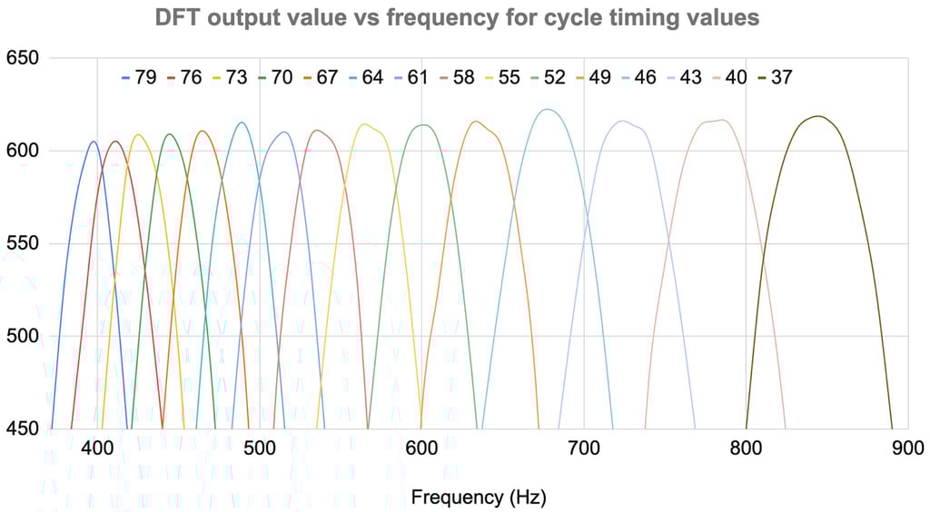
I have included the Goertzel algorithm modules in this category as these are responsible for extracting the carrier level from the incoming signal. The Goertzel calculation runs every 8th timeslot and the output values are produced every 64th timeslot (32 samples per output and 4 parallel processes).
The Goertzel algorithm is "tuned" to the carrier frequency by changing the sampling frequency. This means that the algorithm can be simplified and removes the need for floating point arithmetic which is too slow to fit into a timeslot. The downside is that this means that the timeslots get shorter for higher carrier frequencies. but this is accounted for in the allocation of modules to timeslots.
The frequency response of the Goertzel output for each of the programmed timeslot periods (μs) is shown below.
CW
The CW decoding is broken down into 6 modules which execute sequentially each time a new Goertzel output is produced. The carrier state detection module (CSD) runs first to detect the high-low and low-high transitions. This includes a number of checks to avoid false triggers and produces the high/low state time as an output.
The timing modules (CLT & CHT) extract the minimum low and high times respectively and use these to calculate the thresholds that determine whether a high time is a dot or dash and whether a low time is a symbol, character or word gap. These thresholds need to change dynamically to track changes in the data timing but also maintain some stability to filter out spurious timing anomalies that can cause a cascade of errors. The timing refinement module (CTR) does some of this filtering and also adjusts the thresholds to take account of uneven high/low bit times and long/short inter word and character spaces.
The remaining CW modules generate the CW code for character output and add spaces for word breaks as appropriate. These codes are put into a buffer for output to the display by the next module.
Display
A single display module runs continuously every 8 timeslots to take character codes from the buffer and send them to the display. This is done in 8 stages, each setting 1 bit at a time, to avoid exceeding the timeslot processing time, with a counter used to keep track of the current stage. The LCD display uses a 4 bit interface so a write enable pulse is sent every 4 stages to complete the data transfer.
Controls
This final category includes the modules for the user controls and indications which are limited to a single push button and a tricolour led.
The button allows the character display to be paused to note down relevant details and a second press resumes the display. There is no character buffer in this version though so any characters sent during the pause will be lost.
The signal level indicator (SLI) module takes an output from the signal level measurement module and sets the colour of the led to indicate if the input signal volume is within the range for decoding. This allows the user to adjust the source volume accordingly.
Schedule timing
It is important to ensure that the code in a timeslot does not take up more time than the current ADC period. This would cause the sampling intervals to be irregular and would disturb the output from the Goertzel algorithm. By avoiding the time consuming instructions such as real-time arithmetic, I was able to keep each module down to 10-20μs. As a final check I incremented a test variable in the loop that waits for the period time to expire and checked that this executed at least once in each timeslot.
I have now proved that this program methodology and structure can successfully decode a wide range of CW audio. The next part will look at performance examples and limitations.
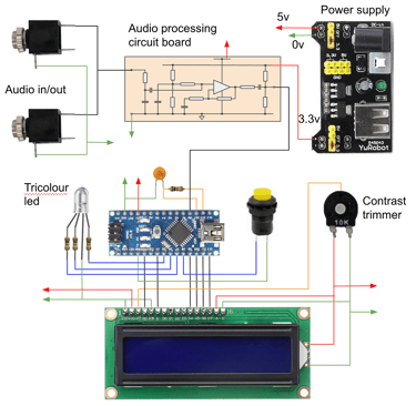
Hardware
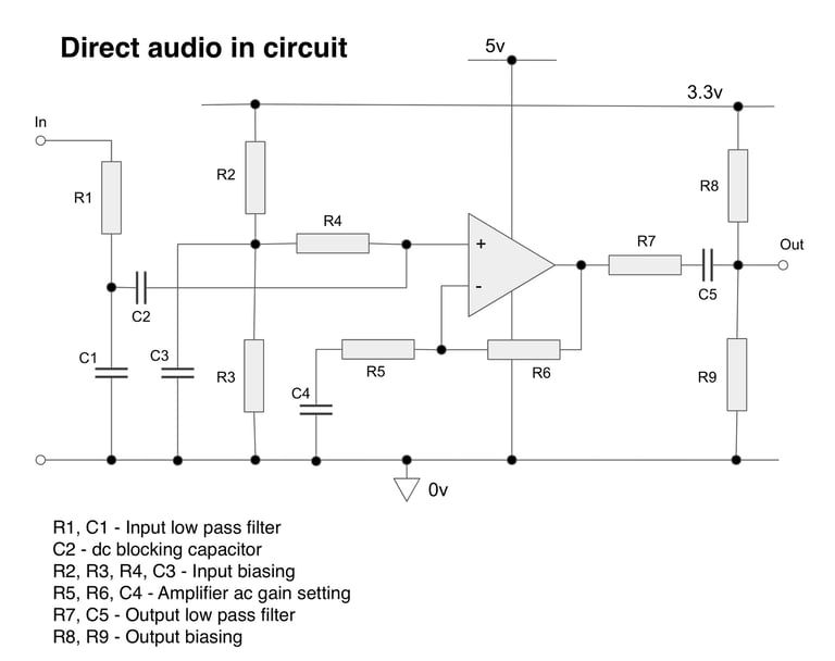
The schematic diagram shows all the components and connections for the decoder.

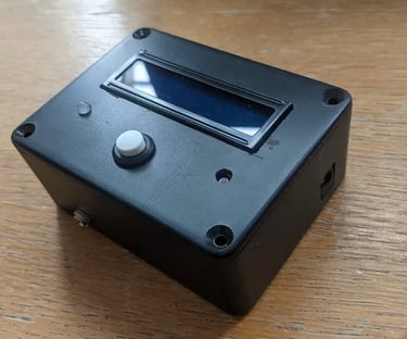
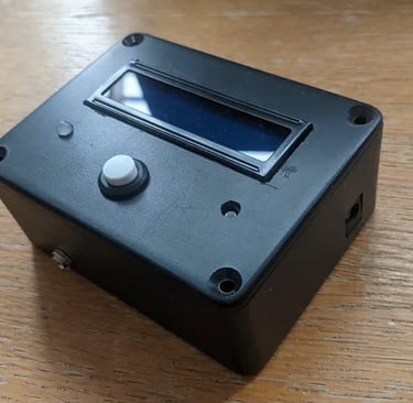
Enclosure
The decoder components fitted comfortably into one of the plastic boxes that I use for my antenna matching transformers. I cut a hole in the lid for the LCD display and arranged the location of the other components around that.
To minimise the wiring and mounting requirements, I piggybacked an Arduino Nano onto the back of the LCD display. By choosing the data pins appropriately, I was able to align them with the matching data connections on the LCD display and use header pins to solder them together and support the Arduino. The LCD display was then secured in the cut-out using double sided sticky pads.
The audio connectors, audio interface board and power supply mounted in the bottom of the box
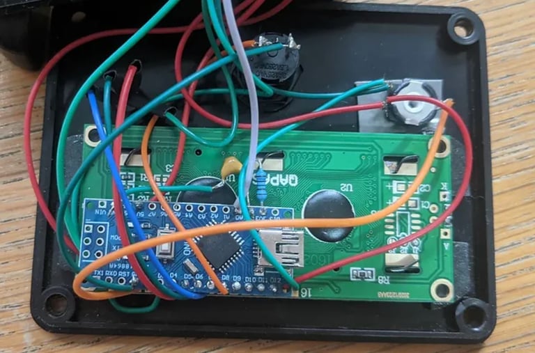
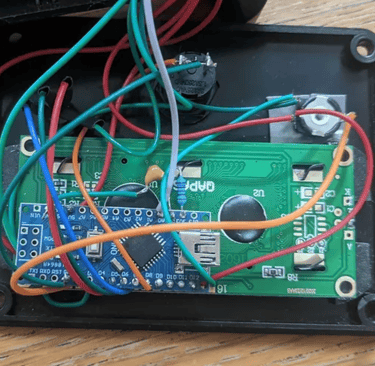
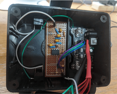
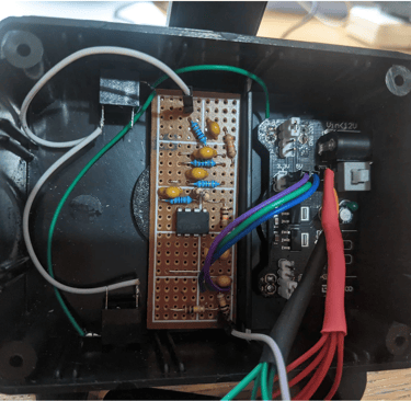
The Arduino Nano mounted on the LCD panel on the inside of the box lid
Performance and limitations
Although I am still refining some aspects of the code, the primary objectives have now been completed and I have a working CW decoder with a few limitations.
I have tested the decoder on a wide range of YouTube videos, web SDR sites and with my transceiver. I have not published any of the live conversations as I believe that I should get the participants permission to do that.
The decoder works with 100% accuracy on the learning videos that I found including speeds of 15 - 38wpm and a wide range of timing variations. The limitation of these is that the signal is virtually noiseless and consistent throughout so once the decoder has picked up the carrier frequency and the speed, it doesn't need to make any changes.

For the Titanic audio (shown here) the decoder is about 99% accurate with a few errors when the decoder retrains to a new transmitter. with a different signal frequency. There is also a section where multiple transmissions are happening simultaneously. The video transcript declares this as "jamming" but my decoder manages to decode the stronger signal for a good part of this section.
The real conversations which some users record and publish tend to have higher noise levels and fading signals. The decoder can now cope with these but will stop when the signal is below a minimum level or the noise level is too high relative to the signal. The same is true of my HF transceiver and web SDR but with the added complication of automatic gain control which brings the noise level up in the gaps between transmissions. This caused quite a few problems at first but I have now implemented algorithms to distinguish between noise and signal and to apply a digital "squelch" to suppress the attempted decoding of noise.
I have addressed many of the limitations in a new cw decoder project using an ESP32 processor and a much better display.
Downloads
The Arduino source code is available to use and modify. It was written using the Arduino IDE and was last updated on version 2.3.0 of the IDE. Please note the code is not professionally written or documented but I am happy to answer any questions that may arise.
The downloads button will open the Pro Antennas Google Drive in a new tab and the relevant file (CW_decoder_pv5_2) can be downloaded by clicking on the 3 dots at the right of the file details and selecting download.
Support
proantennas@gmail.com
+44-7470 337050
© 2025. All rights reserved.